IMPORTANT: This guide covers the generic approaches to modelling in Mira ABM for equities, bonds, long-term scenario analysis and short-term stress testing. Specific underlying models of institutional clients are based on the on-boarding discussion and reflect the modelling choices of users.
¶ General approach to modelling
LINKS Mira ABM methodology combines a value-based asset pricing framework – Graham Risk and an Agent Based Model (ABM) to arrive at short- and long-term return expectations for asset classes and portfolios. Graham Risk, named after Benjamin Graham – the founder of value-based investment doctrine, is an Internal Rate of Return-based metric that compares expected cash flows with the current price paid for the investment. Throughout the application of Mira methodology there is an assumption made that markets can remain over-/undervalued for extended periods of time. Mira’s ABM, on the other hand, is used to assess how the uncertain cash flows may change given real or scenario-based shocks in different parts of the global economy.
As this high-level schematic of Mira’s methodology suggests, Graham Risk derives the value of assets in the world “as it is now”, whereas Mira’s ABM module changes the cash flow profiles, including the profitability of the underlying companies, default rates of corporate bonds and expected long-term growth rates of the economy, after which Graham Risk is used again to arrive at alternative pricing.
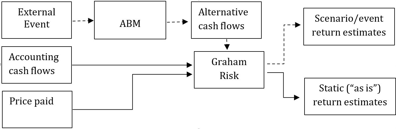
Graham Risk (GR) captures the risk of overpricing; GR for sovereign bonds and regional equities are the primary investment risk drivers. Implicit risk in all other asset categories is mostly derived from the applicable equity/bond GRs. While there may be many different models underlying calculation of Graham Risk for for a particular asset category, the calculation of expected returns based on GR is the same for all asset classes.
Since GR framework has been developed specifically for such distressed environments, it is safely assumed that all equity-related asset classes have the single common driver – equity risk appetite, gauged by GR equities. In practice, this means that should equity GR flag high risk, a similar signal will be expected for high yield, property and all other enterprise risk category assets, except when such asset prices already reflect poor market conditions.
Graham Risk generically is defined as the difference between fair and actual (implied) internal rate of return:
GR = IRR (Fair)-IRR (Actual)
¶ Example (Graham Risk):
The case of a sovereign bond yield is the simplest to demonstrate the meaning of GR. We can estimate based on a Macroeconomic or Statistical approach a certain long-term fair level of interest rate on a 10-year government bond, which incidentally is the IRR of the bond, at say 3%, i.e. IRR(Fair) = 3%. If the current yield of the bond (IRR(Actual)) is 2.5%, the bond's GR = IRR(Fair) - IRR(Actual) = 3% - 2.5% = 0.5%. This means that the bond's yield is 50 basis points below its fair level. Assuming the bond's duration is 7.5 years, the expected correction in price due to valuation (as the bond's price goes up so as to bring the yield up by 50 basis points) is - Duration x GR, i.e. -7.5 x 0.5 = -3.75%. Therefore, GR is an IRR-based measure of over-/under-pricing.
¶ Modelling bonds, interest rates
Calculating GR of a bond (the difference between the fair and currently observed yield) assumes that we know the fair level of the yield. Mira ABM uses a factor-based model to estimate the fair yield. More specifically, Mira follows a strict procedure to establish a reliable historical relationship between the variables that explain yields (explanatory variables) and the yields:
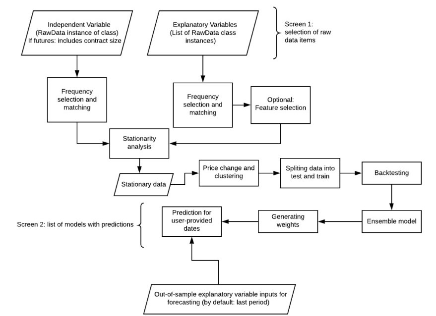
While the exact definition of models is beyond the scope of this guide (though it is available to our clients upon request), the procedure is designed to avoid establishing random (spurious) relationships. The procedure is also model-agnostic in a sense that we employ multiple statistical models and the procedure selects the results on the basis of each model's forecasting ability.
Another, more important safeguard is the common sense approach to modelling:
- All explanatory variables should have an economic rationale
- Relationships should exist consistently across time and regions.
A typical standard factor model for the European 10-year generic bond yield would have the following factors:
- EUROSTAT Gross Household Saving Rate - Eurozone SWDA
- ECB Eurozone Employment YoY SA
- OECD Euro Area Early Estimate Productivity Change YoY
- Eurostat Eurozone Core MUICP YoY
Factors change from region to region, depending on the availability of data and relevance. At the same time institutional subscribers during the on-boarding process have the option of changing the list for every asset category.
An additional and very specific non-optional factor is Return on Equity (ROE). For European sovereign bonds we use aggregated ROE of 400 largest European stocks. This allows us to establish an empirical relationship between the companies (businesses) and government bond yields.
Based on the actual application of the model and having a set of explanatory variable value sets, we can determine a "fair level" of yield. By default, if there are no World Views implemented, these values are set at their most recent observations. This means that the most recent reported values of productivity, employment, CPI, savings rate and ROE would define the fair level of yield.
Actual observed yield and duration of the bonds used in Mira ABM are directly imported from data providers for each benchmark. Using the fair and actual levels of yields, Mira calculates the GR and the correspondent return expectations.
¶ Types of return expectations
There are several "types" of returns in Mira ABM that may appear to be contradictory at times. Return calculation in Mira is based on the GR value and duration. Returning to the earlier example of a bond with a current yield of 2.5% (Y), duration of 7.5 (D) years and GR of 0.5%(GR), we would expect this bond's yield to increase by the value of GR (i.e. current yield will tend to the fair yield).
By default, Mira assumes that the valuation correction happens within the first three years (this may be different if you have customised models). So the first three years, we would expect the bond to post losses of principal value of:
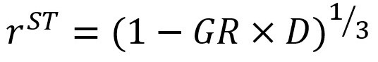
This is the short-term return expectation from the bond. The equation is not complete, though, as apart from the loss of principal value, the bond will keep yielding. Also, the initial value loss (-GR x D) is only an estimation for small values of GR. With larger values, we need to incorporate a convexity component (C):
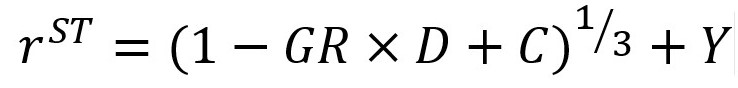
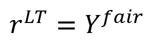
After the change in the principal value (valuation adjustment), the instrument's return becomes equal to its fair yield, so the long term return is the same as fair yield.
Finally, Mira ABM separately reports the instant impact or +/- valuation, which is the total value gain/loss due to change in valuation. This is nothing other than the -GR x D term of the equation for short-term return.
The three types of return (short term, long term and valuation) are represented here in the third, fourth and last columns:
¶ Modelling equities
Modelling equities adds an additional layer of complication, as the cash flows of equities are uncertain. While in case of bonds, we could estimate the fair level of yield and compare it to the actually observed yield, in case of equities, Mira ABM estimates both the fair Equity Risk Premium (ERP) and the current level of ERP given the expected cash flows.
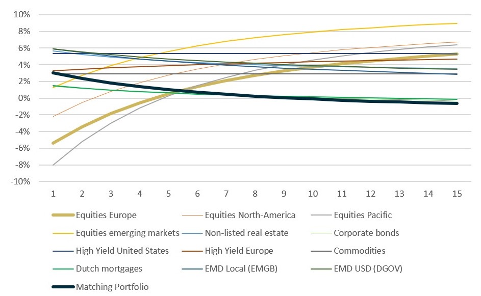
The actual model underlying the equity asset categories in Mira ABM may differ due to client preferences and available data, however, the generic model is given by:
In order to estimate GR for equities, Mira ABM first calculates historical time series of ERP's then runs a historical analysis almost identical to the one used in bonds (see Modelling bonds, interest rates), albeit with different factors.
IMPORTANT: The fair level of ERP depends only on the macroeconomic drivers and not the ROE. Short-term stress tests that result in different levels of ROE, therefore, change the current Equity Risk Premium and not the fair one. The fair Equity Risk Premium changes only when one of the factor values is changed in the World Views.
By default, the equity model uses trailing 12=month observed Returns on Equity (ROE) as the key input in estimating the ERP. These data are updated in Mira ABM on the weekly basis, using bottom-up aggregation by region. For instance, in the midst of the earnings season, the companies reporting during the week will be reflected in the ROE the week after. If the reports are stronger compared to the previous ones, the aggregated ROE will increase, which if market prices do not change, will result in higher current ERP. As the fair level of ERP does not change, this will result in lower Graham Risk (ERP fair - ERP current), which means equities will be valued higher and will have higher upside potential.
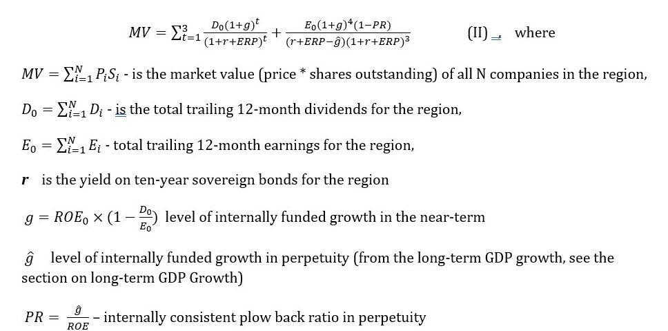
For most equity models, Mira ABM gives the detailed overview of underlying data. In the Dashboard or Scenarios view, click on the Equities model and select Inspect in the top right corner:
In this case, for instance ROE of 9.2% is used for calculation, which is the same as the scenario ROE, as this calculation is "no-stress".
¶ World Views: long-term assumptions
World Views in Mira ABM are a collection of settings/assumptions that drive long-term asset pricing. As fair level of yields, spreads, equity risk premiums are estimated using factor-based models, the actual values depend on those factor loadings. For instance, if we knew the level of employment, inflation, productivity growth rates and savings rates, we would be able to arrive at the appropriate government bond yield using the factor model. World views help establish those inputs.
The difficulty with setting these assumptions, however, is that it may not be easier than setting the yields explicitly. Translating the yields into factors, for instance, assumes that we have a better idea about the factors than the yields. However, it would be difficult for most users to expressly set values for savings, productivity etc. This is why, World Views are structured based on a certain hierarchy:
World Views -> Long-Lasting Trends -> Choices
Each World View consists of a number of Long Lasting Trends that in turn consist of Choices.
IMPORTANT: Long-Lasting Trends are observable and clear social trends that occurred in the past, continue to occur in present and with a high level of confidence will continue to occur in the future, albeit possibly with varying intensity.
Examples of Long-Lasting Trends in Mira ABM are:
- Ageing Population
- Automation
- Climate Change
- Globalisation and Trade Tensions
- Monetary policy
- Regional Competitiveness
A specific feature of long-lasting trends is that they directly and strongly affect the factors used in modelling interest rates, equity risk premiums and spreads. For instance, aging population impacts the number of people in the retirement age, which directly impacts the number of savers and the savings rate in the economy. This relationship does not require statistical analysis, but a simple arithmetic calculation.
By using Long-Lasting Trends, Mira ABM enables users to set the values of factors with greater confidence.
World Views are set in the World Views tab. By default there may be a single World View set, however, users may add, delete and edit World Views:
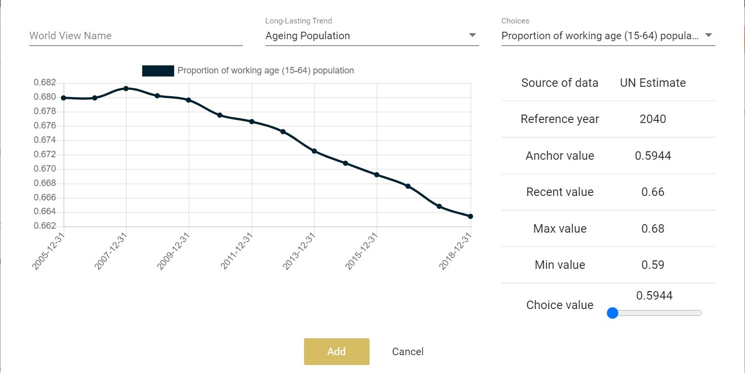
The menu of World Views gives basic information about each choice, including the historical values in a graph (if they are available), lowest and highest values, an anchor value, which is either an estimate from a reputable source, or the most recently observed value.
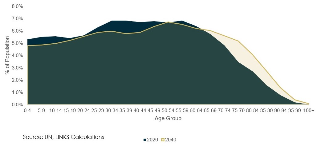
¶ Ageing Population
A great feature of Ageing Population as a long-lasting trend is that it is entirely predictable. Reliable estimates of the proportion of working age population in 10-30 years come from the United Nations:
There is only one Choice in Ageing Population LLT: the Proportion of Working Age Populaton
As the proportion of working age population shrinks, conversely, the proportion of retired population increases, which impacts:
- Gross Household Savings Rate: retired population does not save (evidence from EU and the US), so an increase in the proportion of retired population results in proportionate decrease in the savings rate (s = s(recent) x (1 - delta_aging/number_of_years).
- Total Employment: directly impacts growth rate of employment
To the extent that the underlying bond and equity models use these savings rate and total employment as factors, changing the pace of ageing population will change the factor loadings and impact the fair level of yields and Equity Risk Premiums.
Important: Although the actual pace of ageing may not be debatable, the setting in Mira ABM refers to the proportion of working age population, which is affected by how late people retire. So a good way to think about this is that the setting refers to the policy decision of retirement age, rather than the actual age composition of the population.
¶ Automation
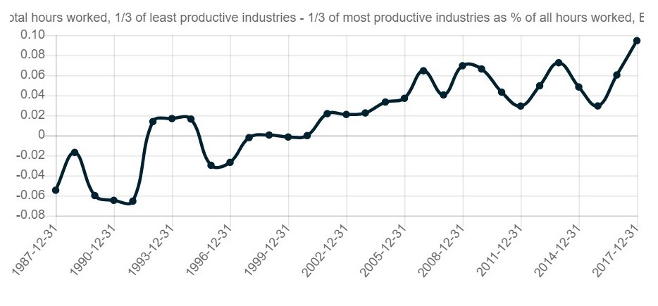
The trend of automation is another long-lasting trend that is easy to predict and assume that it will continue in the future. The specific aspect of automation that Mira focuses on has to do with economy-wide productivity. Although based on conventional wisdom, automation should improve productivity, a specific feature of automation in the past two decades is its uneven application: some industries, such as manufacturing, energy, utilities have been beneficiaries of very fast automation, while others, such as education, services have lagged behind. As a result, we have seen employment migration from more productive industries to less productive industries.
In the graph below, Mira calculates the difference in proportion of employees (as % of total employment pool) engaged in the least productive industries vs. most productive industries. Every year, industries are ranked based on productivity (value per employee) and split into three buckets. The graph shows the difference in percentage of employees engaged in the top bucket vs. bottom bucket. Clearly, while in the 1980s and 1990s industries with higher productivity employed more people, over time people migrated into the low productive industries, and as they did that, their productivity declined. The combined effect of this process dampens the productivity growth rate for the whole economy.
There are two choices that can be set in this LLT:
- Choice 1: Future expected value of the migration, i.e. % of people engaged in low productive industries vs. high productive industries
- Choice 2: Percentage of people (of those who quit the high productive industries) that fail to migrate, i.e. drop out of the labor pool permanently.
These choices are directly connected to the following factors:
- Productivity growth rate: economy-wide productivity growth rate for the next 15 years will have a direct calculable impact (Mira splits the productivity growth rate into the high- and low-productive parts and calculates new values of productivity based on the input) on overall productivity growth rate
- Employment growth rate: people dropping out of employment pool will have a direct impact on employment growth rate (recent value will be decreased by the target value of drop-outs by year).
Asset class models that depend on the productivity growth rate and employment growth rate will have their fair values impacted by the settings.
¶ Globalisation and Trade
Globalisation level impacts the ability of companies to source raw materials/inputs cheaper and sell their products globally. Trade as percentage of GDP is the main metric used here:
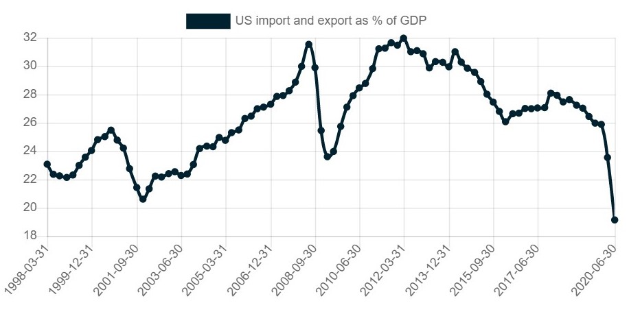
Mira establishes a historical relationship between the ROE's of European and US companies and the level of globalisation as expressed by trade as percentage of GDP. Any change in the globalisation assumptions leads to an impact on ROEs in Europe and the US.
¶ Monetary Policy
Monetary policy, more specifically errors in monetary policy result in unsustainably high or low inflation rates. The fact that inflation (CPI) has been relatively steady and low is a long-lasting trend that may or may not break in the future. In this section, users can set background inflation expectations by region:
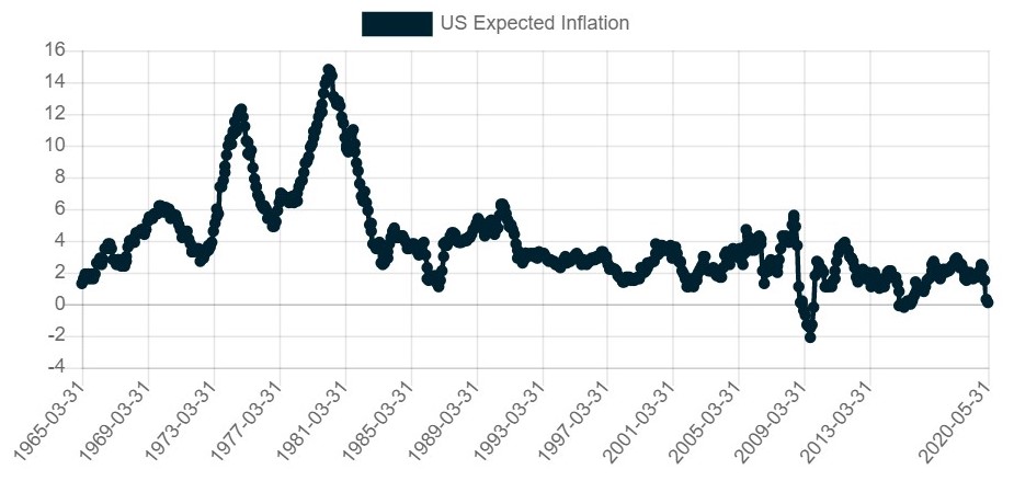
Asset categories that use rates of inflation as a factor, will be impacted by the change in the level of expected inflation.
IMPORTANT: Apart from exogenous inflation, which is the demand-driven inflation, Mira ABM handles also endogenous inflation caused by supply shocks - supply-driven inflation. This type of inflation is short-term in nature and is a result of price level changes due to the Agent-Based Modelling (see the next section). In other words, short-term stress test related inflation in Mira ABM is an outcome, rather than an assumption.
¶ Climate Change Transition
Climate change transition in Mira ABM is modeled along the assumptions of the Dutch National Bank (DNB), however, with bottom-up methodology that is more applicable in Mira ABM.
The impact of Climate change transition assumptions are linked with regional ROE rates. These directly impact the short-term ERP calculations, but also fair level of bond yields and spreads. There are two choices in this LLT:
- Technology shock: the impact of transition to new business models and technologies in order to combat climate change. The three settings (minimum, average, extreme) correspond to three different paces of transition.
- Policy shock: separately, application of a policy shock would mean a $100 per ton of CO2 tax across all industries and geographies.
For more on climate change modelling in Mira ABM and the underlying assumptions please consult the Risk Wire document.
¶ Regional Competitiveness
ROEs by region in Mira ABM are treated as a long-lasting trend, since they are relatively stable or trending and depend on clear and predictable political and economic developments: degree of regulation, education, technological advantage, availability and quality of labor etc. Setting ROEs explicitly allows for judgement calls with respect to those socio-economic trends. If the users have no specific views, it is prudent to set ROEs at average (cross-cycle) levels.
Setting ROEs impact not only equities, but also spreads and government bonds, as ROEs are factors in fair yield assessment.
¶ Saving World Views and Running Calculations
Once a World View is saved, you can access a summary of that World View's impact on factors. Each row of the table is a factor used in the system, wile each of the columns is a long-lasting trend. The total impact on the actual value used in calculations is summative; it is a simple summation of all impacts across all LLT's:
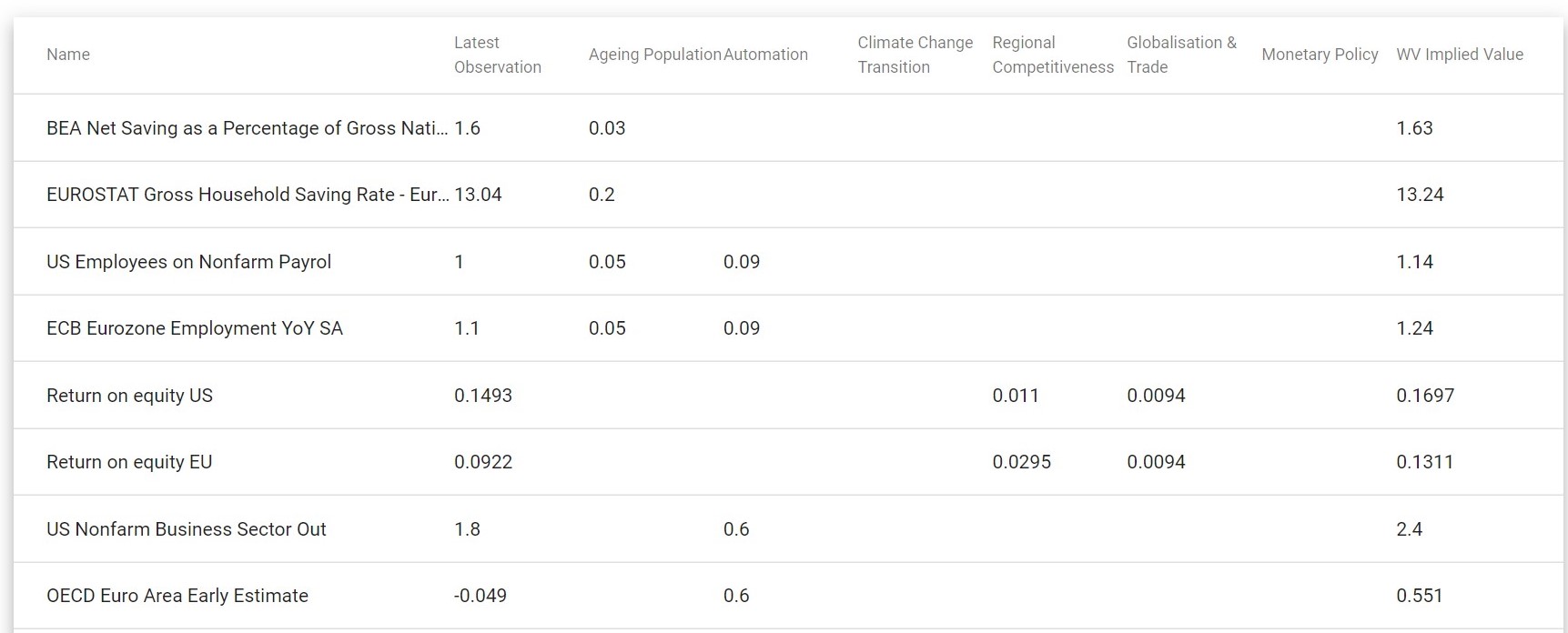
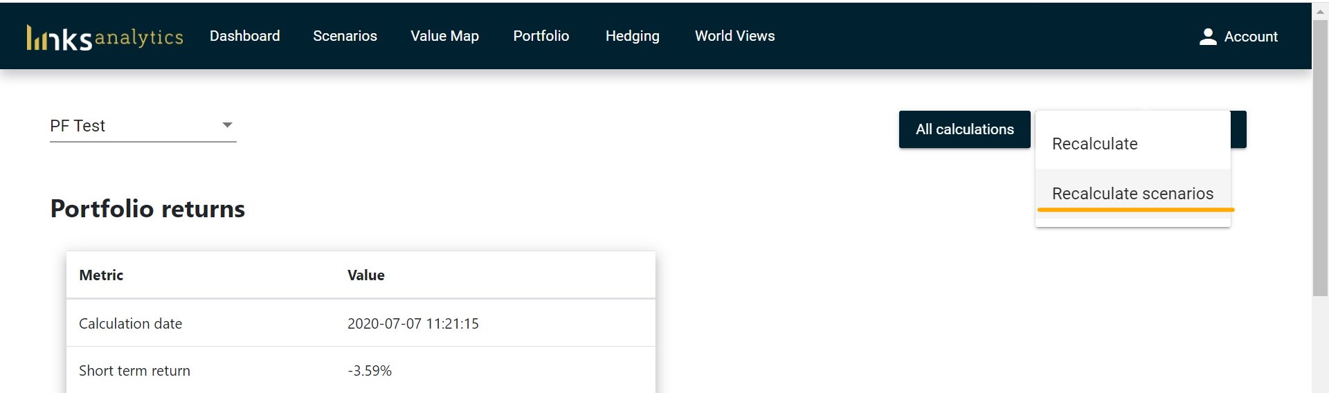
In order to use the World View in your calculations, you need to select it from the drop-down menu and click on Set as Default. If you then go to the Dashboard and recalculate your portfolio, it will use the new World View.
VERY IMPORTANT: ABM-based short-term stress test calculations in Scenarios also use the default World View. If you change the default World View, your impact values in Scenarios will still be based on old default World View and will be meaningless. If you want to align the Scenarios with the new World Views, you will need to recalculate them too. This can be done by clicking Recalculate scenarios in the Dashboard:
¶ Scenarios: Agent-Based Modeling and stress tests
Short-term stress scenarios in Mira ABM are handled by the Agent-Based Modelling (ABM) module. The underlying data of ABM come from country-specific input-output matrices, WTO trade data and other industry-specific data sources. Mira ABM database consists of 40 countries and 70 industries in each country.
Most stress tests that are potentially a concern for institutional investors are short-term in nature (e.g. Brexit, Covid-19, Currency or commodity-based routs etc). Historical statistical analysis is not effective in estimating the impact of these events, since they have no historical precedents. ABM simulates economic activity forward on the basis of the initial shock. The result of simulation is then aggregated to yield ROE and price-level changes by region that are then used to estimate the impact by asset class.
The formal model definition is as follows:
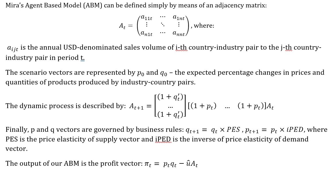
¶ Defining Scenarios
A scenario definition in ABM consist of sets of country/industry price and/or volume shocks.
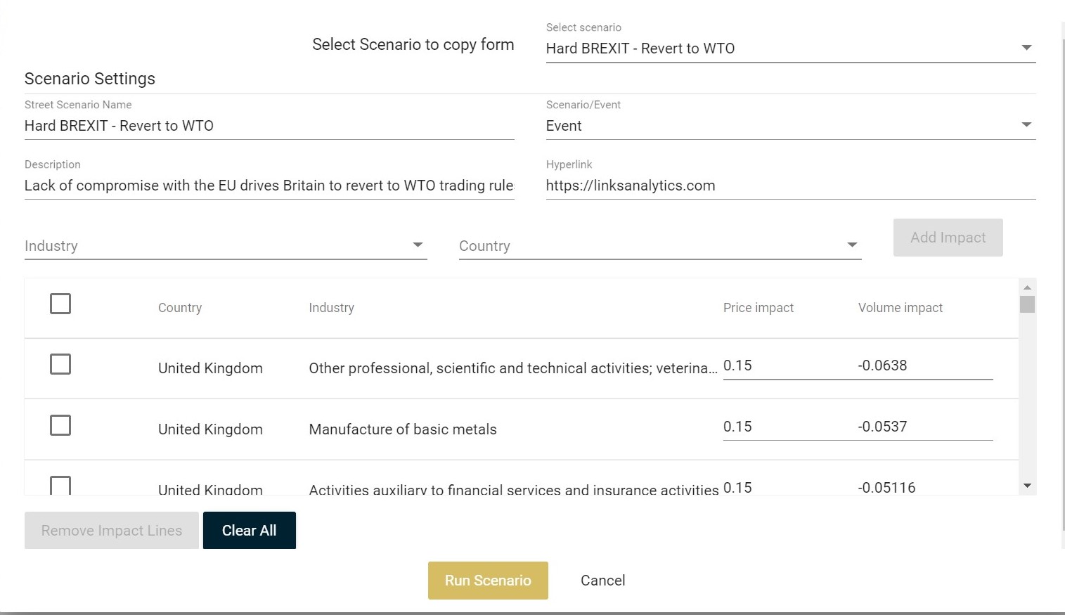
Nearly all stress scenarios can be distilled into price and volume impacts by industry and country. An oil price decline, for instance, can be modeled as price change in all oil industries across all oil producing countries. An easy place to start is to copy from some of the existing scenarios.
While users can add their own scenarios to their portfolios, LINKS adds frequently scenarios across all client portfolios. These can then be copied and amended as required.
IMPORTANT: The list of scenarios in the Scenarios tab cannot be amended or changed. The most recent scenarios are added to the list at the top. If you want to amend a scenario, you can copy from existing and add a new one.
¶ Interpreting the Results
The instant value impact of scenarios on the portfolio is given at the top right of the Scenarios tab:
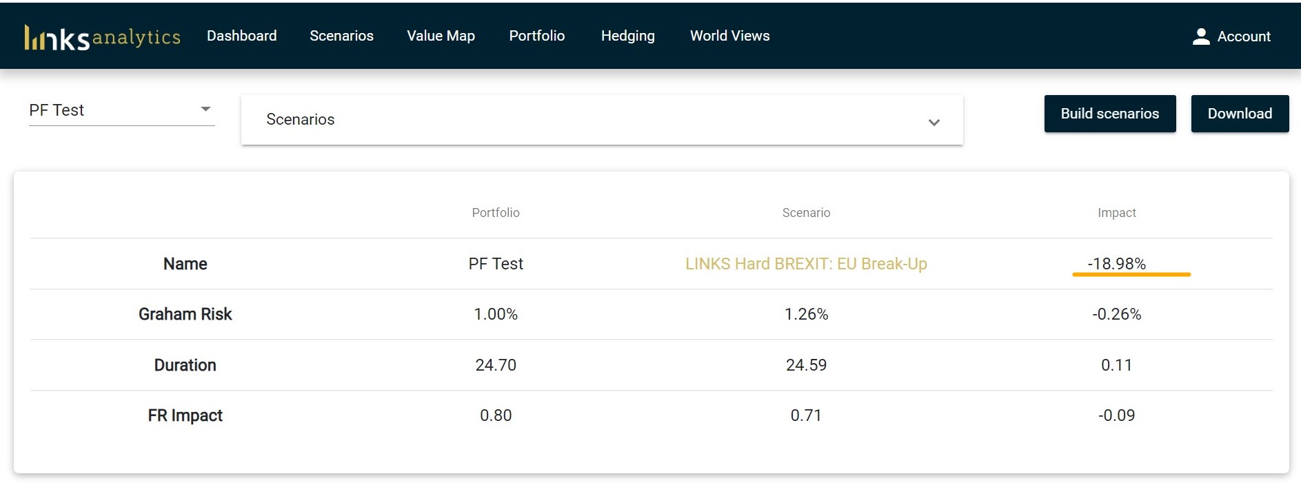
The Impact here is assumed to be short-term or instant, i.e. this is the change in Net Present Value of all investments. Since the stress tests are short-term, it is not possible to pinpoint the exact timing of the impact.
If the portfolio has liabilities included, there will also be an impact on Funding Ratio (last row).
You can use the Inspect functionality to understand the impact of ABM across asset classes. In Scenario tab the Inspect functionality yields the impact of the scenario on profits and prices across regions:
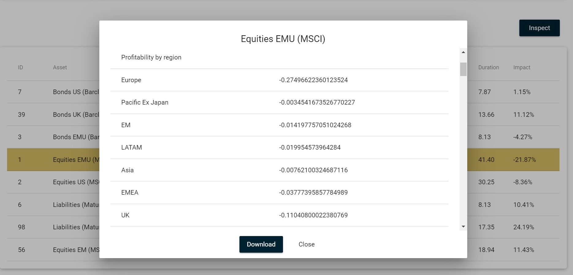
Further down the inspect list you can see how the changes in price and profitability level are integrated with pricing of each asset you select.
More information on the scenario is available by clicking on the Name of the scenario in the Scenarios tab. The first table in the detail picture is a list of scenario inputs.
The sankey diagram needs a specific interpretation:
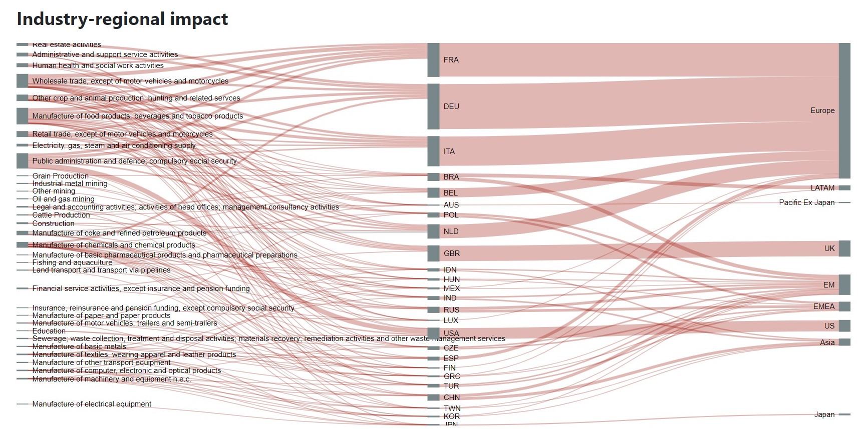
The diagram is used to demonstrate the industries, countries and regions that had the greatest impact from the scenario. The thickness of lines is the absolute USD value of the impact.
IMPORTANT: Note that since the size of the impact is in USD, it is not relative to the economy's size. So a small impact in say Greece could mean a very large impact relative to the size of Greece's economy.
Most scenarios have both positive and negative impacts, so positive values will be shown in grey, while negative values are in pink. Positive and negative values are not cancelled out, but rather stacked together. This means for one country you may see a stacked grey line on top of a pink line. The net impact is of course the difference between the two, but the diagram helps you to understand the composition of impacts.
Finally, the last table in the details section shows the impact of the scenario on yields, spreads and Equity Risk Premiums of the underlying asset classes.
¶ Further reading
Please consult our Methodology section for further reading or get in touch with us with specific questions. A very useful source of information is our online training course:
Resetting the Investment Process in the Age of Disruptions